10.8 Metabolomics Single-Omics Quick-Start Example

This section demonstrates a complete and commonly used analytical workflow for metabolomics data, from data import to functional interpretation, using example datasets.

Example data download: Github link

10.8.1 Importing Metabolomics Data

library(EasyMultiProfiler)


meta_data <- read.table('col.txt',header = T,row.names = 1)
data <- read.table('metabol.txt',header = T,quote = '',sep = '\t')

MAE <- EMP_easy_import(data = data,coldata = meta_data,
                       sampleID = rownames(meta_data),
                       type = 'normal')

10.8.2 Exploring Metabolomics Data

View Current Metabolomics Assay

MAE |>
  EMP_assay_extract() # View abundance matrix

MAE |>
  EMP_coldata_extract() # View phenotype data

MAE |>
  EMP_rowdata_extract() # View metabolite annotations

10.8.3 Calculate Coefficient of Variation for Quality Control (Optional)

Compute CV for Metabolite Features Using QC Samples

MAE |>
  EMP_assay_extract() |>
  EMP_mutate(CV = sd(c(QC1,QC2,QC3,QC4,QC5,QC6))/mean(c(QC1,QC2,QC3,QC4,QC5,QC6)),
  mutate_by = 'feature',location = 'rowdata',action = 'rowwise',.before = 2)

Filter Metabolites Based on CV

MAE |>
  EMP_assay_extract() |>
  EMP_mutate(CV = sd(c(QC1,QC2,QC3,QC4,QC5,QC6))/mean(c(QC1,QC2,QC3,QC4,QC5,QC6)),
             mutate_by = 'feature',location = 'rowdata',action = 'rowwise',.before = 2) |>
  EMP_filter(feature_condition = CV < 0.3)

10.8.4 Aggregate Metabolite Data by Phenotype Annotation

Collapse Metabolites by Metabolite Name

MAE |>
  EMP_assay_extract() |>
  EMP_collapse(collapse_by = 'row',
               estimate_group = 'MS2Metabolite')

Collapse Metabolites by KEGG ID

MAE |>
  EMP_assay_extract() |>
  EMP_collapse(collapse_by = 'row',
               estimate_group = 'MS2kegg')

10.8.5 Metabolite Identifier Conversion

The EMP package supports cross-database metabolite ID conversion, including CAS, DTXSID, DTXCID, SID, CID, KEGG, ChEBI, HMDB, and Drugbank.

MAE |>
  EMP_assay_extract() |>
  EMP_collapse(collapse_by = 'row',
               estimate_group = 'MS2kegg') |>
  EMP_feature_convert(from = 'KEGG',to = 'HMDB')

MAE |>
  EMP_assay_extract() |>
  EMP_collapse(collapse_by = 'row',
               estimate_group = 'MS2kegg') |>
  EMP_feature_convert(from = 'KEGG',to = 'Drugbank')

10.8.6 Batch Effect Correction (Optional)

MAE |>
  EMP_assay_extract() |>
  EMP_adjust_abundance(.factor_unwanted = 'Region',
                       .factor_of_interest = 'Group',
                       method = 'combat_seq')

10.8.7 Metabolite Abundance Normalization

MAE |>
  EMP_assay_extract() |>
  EMP_collapse(collapse_by = 'row',estimate_group = 'MS2Metabolite') |>
  EMP_decostand(method = 'relative')

MAE |>
  EMP_assay_extract() |>
  EMP_collapse(collapse_by = 'row',estimate_group = 'MS2Metabolite') |>
  EMP_decostand(method = 'clr')

MAE |>
  EMP_assay_extract() |>
  EMP_collapse(collapse_by = 'row',estimate_group = 'MS2Metabolite') |>
  EMP_decostand(method = 'log2')

10.8.8 Differential Abundance Analysis

Wilcoxon Test for Differential Metabolites

MAE |>
  EMP_assay_extract() |>
  EMP_collapse(collapse_by = 'row',estimate_group = 'MS2Metabolite') |>
  EMP_diff_analysis(method = 'wilcox.test',estimate_group = 'Group') |>
  EMP_filter(feature_condition = pvalue < 0.05)

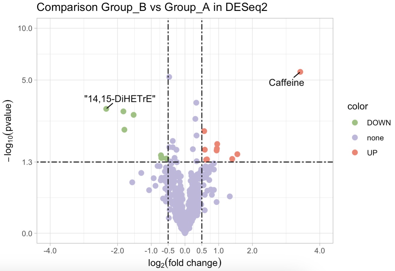
DESeq2 Analysis with Volcano Plot

MAE |>
  EMP_assay_extract() |>
  EMP_collapse(collapse_by = 'row',estimate_group = 'MS2Metabolite') |>
  EMP_diff_analysis(method = 'DESeq2',.formula = ~Group) |>
  EMP_volcanol_plot(key_feature = c('Caffeine','\"14,15-DiHETrE\"'),
                    palette = c('#FA7F6F','#96C47D','#BEB8DC'),
                    dot_size = 2.5,threshold_x = 0.5,mytheme = "theme_light()",
                    min.segment.length = 0, seed = 42, box.padding = 0.5)

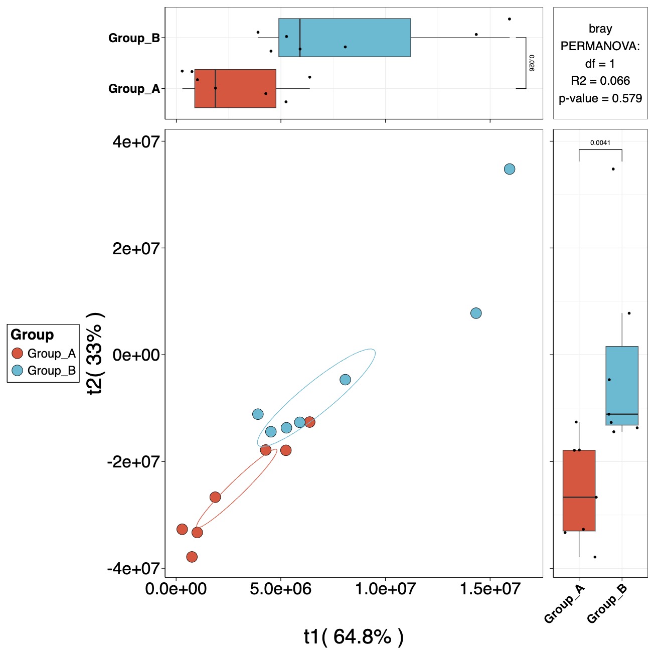
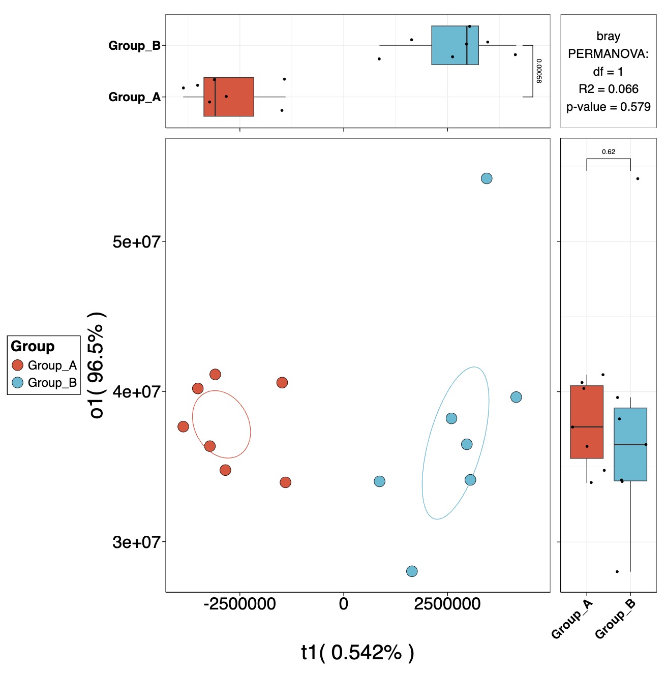
PLS and OPLS-DA Modeling

Calculate Metabolite VIP Scores

MAE |>
  EMP_assay_extract() |>
  EMP_collapse(collapse_by = 'row',estimate_group = 'MS2Metabolite') |>
  EMP_dimension_analysis(method = 'pls',estimate_group = 'Group')

MAE |>
  EMP_assay_extract() |>
  EMP_collapse(collapse_by = 'row',estimate_group = 'MS2Metabolite') |>
  EMP_dimension_analysis(method = 'opls',estimate_group = 'Group')

Visualize Dimension Reduction Models

MAE |>
  EMP_assay_extract() |>
  EMP_collapse(collapse_by = 'row',estimate_group = 'MS2Metabolite') |>
  EMP_dimension_analysis(method = 'pls',estimate_group = 'Group') |>
  EMP_scatterplot(show='p12html',ellipse=0.3)

MAE |>
  EMP_assay_extract() |>
  EMP_collapse(collapse_by = 'row',estimate_group = 'MS2Metabolite') |>
  EMP_dimension_analysis(method = 'opls',estimate_group = 'Group') |>
  EMP_scatterplot(show='p12html',ellipse=0.3)

10.8.10 Identify Key Metabolites

Filter Metabolites Using PLS VIP and Differential Analysis This step filters features by combining results from both differential analysis and dimension reduction, with specific thresholds adjustable based on research needs.

MAE |>
  EMP_assay_extract() |>
  EMP_collapse(collapse_by = 'row',estimate_group = 'MS2Metabolite') |>
  EMP_diff_analysis(method = 'wilcox.test',estimate_group = 'Group') |>
  EMP_dimension_analysis(method = 'pls',estimate_group = 'Group') |>
  EMP_filter(feature_condition = VIP >1 & pvalue < 0.05 & abs(fold_change >1.2))

10.8.11 Machine Learning for Feature Selection

The EMP package includes Boruta, Random Forest, XGBoost, and Lasso for feature selection.

Run help(EMP_marker_analysis) for details.

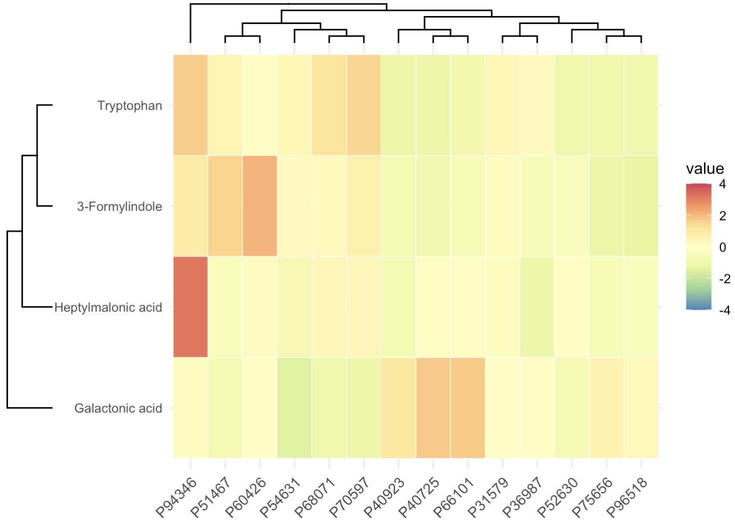
Boruta Algorithm with Heatmap Visualization

MAE |>
  EMP_assay_extract() |>
  EMP_collapse(collapse_by = 'row',estimate_group = 'MS2Metabolite') |>
  EMP_marker_analysis(method = 'boruta',estimate_group = 'Group') |>
  EMP_filter(feature_condition = Boruta_decision!= 'Rejected') |>
  EMP_heatmap_plot(palette='Spectral',legend_bar='auto',
                   scale='standardize',
                   clust_row=TRUE,clust_col=TRUE)

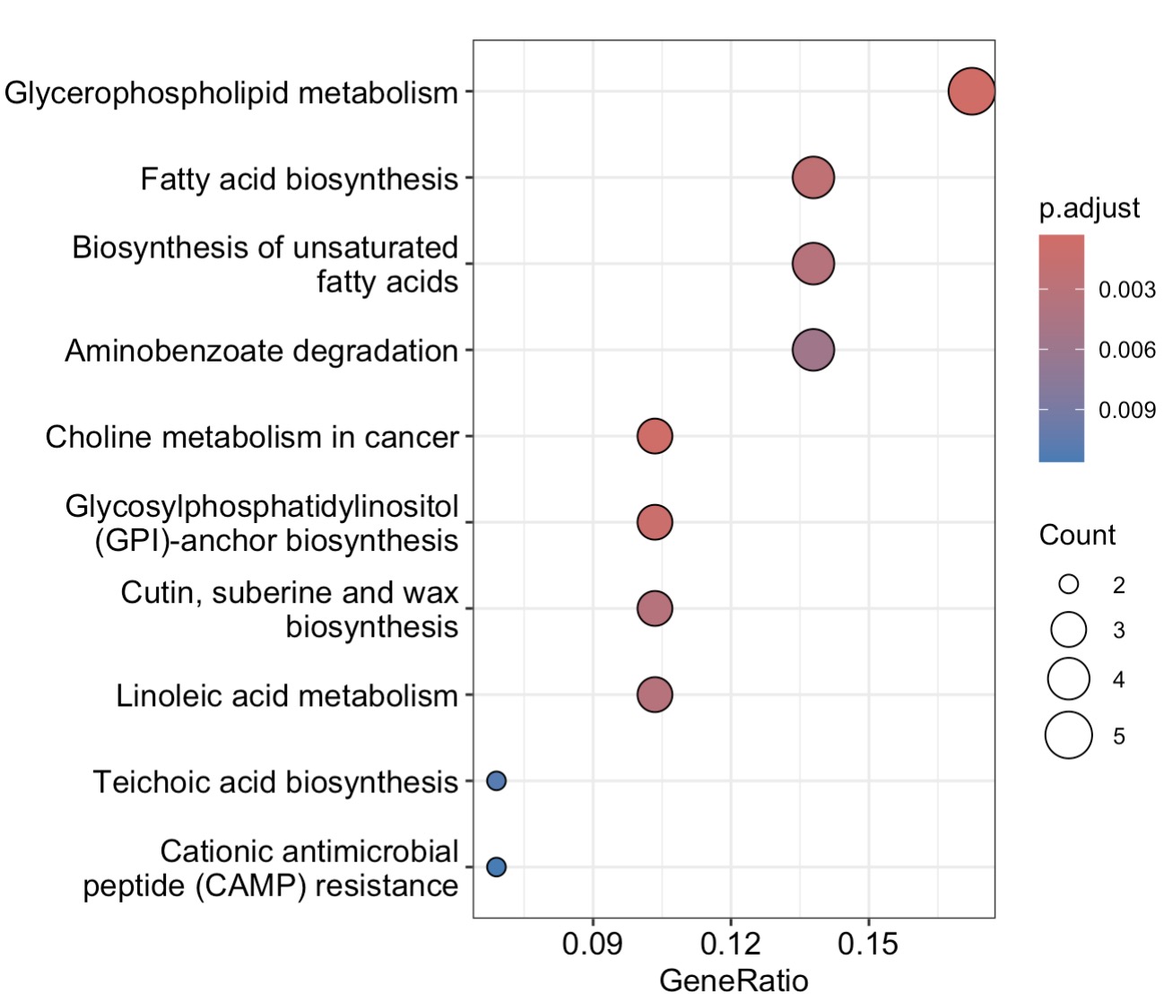
10.8.12 KEGG Enrichment Analysis for Metabolomics

MAE |>
  EMP_assay_extract() |>
  EMP_collapse(collapse_by = 'row',estimate_group = 'MS2kegg') |>
  EMP_dimension_analysis(method = 'pls',estimate_group = 'Group') |>
  EMP_filter(feature_condition = VIP >1) |>
  EMP_enrich_analysis( keyType ='cpd',
                       KEGG_Type = 'KEGG',
                       pvalueCutoff=0.05) |>
  EMP_enrich_dotplot()

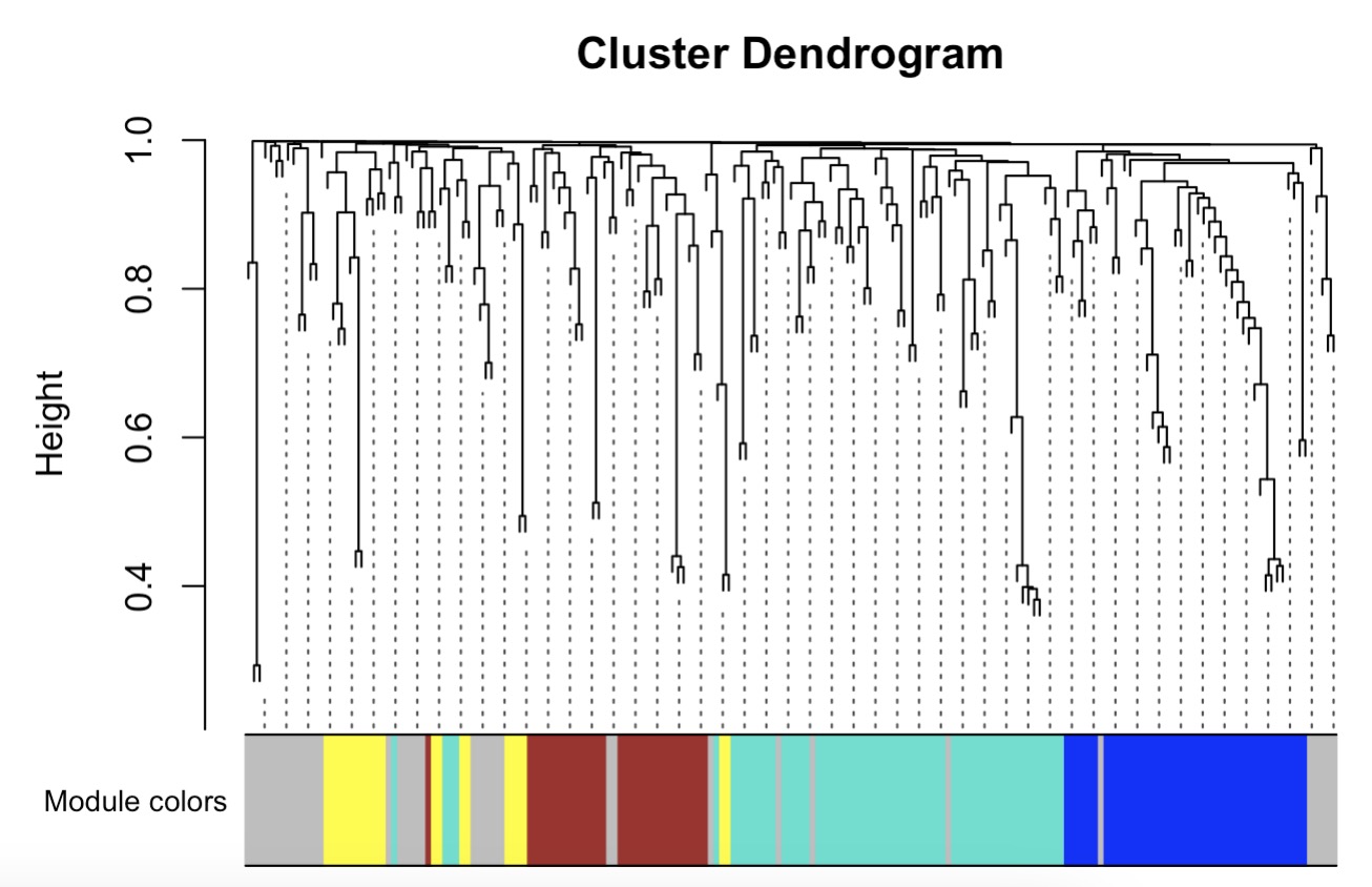
10.8.13 WGCNA for Metabolomics Data

Step 1: Metabolite Clustering Based on Phenotype

MAE |>
  EMP_assay_extract()  |> 
  EMP_collapse(collapse_by = 'row',estimate_group = 'MS2kegg') |>
  EMP_WGCNA_cluster_analysis(RsquaredCut = 0.8,
                             mergeCutHeight=0.2,
                             minModuleSize=10)

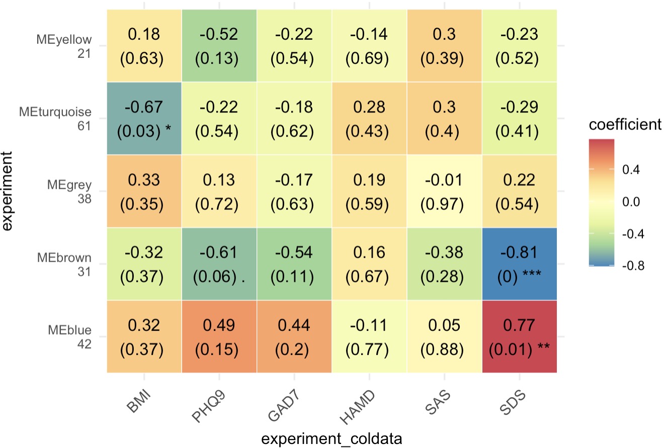
Step 2: Heatmap of Phenotype-Correlated Metabolite Modules

MAE |>
  EMP_assay_extract()  |> 
  EMP_collapse(collapse_by = 'row',estimate_group = 'MS2kegg') |>
  EMP_WGCNA_cluster_analysis(RsquaredCut = 0.8,
                             mergeCutHeight=0.2,
                             minModuleSize=10)  |>
  EMP_WGCNA_cor_analysis(coldata_to_assay = c('BMI','PHQ9','GAD7','HAMD','SAS','SDS'),
                         method='spearman') |>
  EMP_heatmap_plot(palette = 'Spectral')

Step 3: Enrichment Analysis for Selected Metabolite Modules

MAE |>
  EMP_assay_extract()  |> 
  EMP_collapse(collapse_by = 'row',estimate_group = 'MS2kegg') |>
  EMP_WGCNA_cluster_analysis(RsquaredCut = 0.8,
                             mergeCutHeight=0.2,
                             minModuleSize=10)  |>
  EMP_WGCNA_cor_analysis(coldata_to_assay = c('BMI','PHQ9','GAD7','HAMD','SAS','SDS'),
                         method='spearman') |>
  EMP_heatmap_plot(palette = 'Spectral') |>
  EMP_filter(feature_condition = WGCNA_color == 'blue' ) |> 
  EMP_enrich_analysis(keyType = 'cpd',KEGG_Type = 'KEGG') |>
  EMP_enrich_dotplot()

10.8 Metabolite example